Updated October 2026. The code below now splits before fitting a scaler, corrects F1, applies sigmoid before logistic classification, and calculates the appropriate loss. Download the tested NumPy helpers. The original 2021 plots and reported scores are retained as historical output; they do not evaluate the corrected pipeline.
import numpy as npThe two entry level machine learning algorithms , linear and logistic regression are quite easy to understand and provide a good way to practice coding the general machine learning pipeline, in their vectorized form. Namely,
- Prepping the dataset, eg: removing outliers, adding features(polynomial multiples of existing features), normalization, feature scaling.
- Implementing the learning algorithm function.
- Calculating the loss through the chosen loss function and hypothesis.
- Optimization algorithm – Update you model’s parameters depending on the loss and ground truth.
- Maintaining a config file for the total training process.
An entry level toy dataset: pima indians diabetes dataset, has a target of one variable for each datapoint(a binary classification task of predicting whether a person has diabetes or not), will be used for the sake of this tutorial blog.
About the dataset
You can know all about the dataset on Kaggle. The dataset has around 768 datapoints and 8 features, small enough to inspect while practicing a complete learning pipeline. Dataset size alone does not guarantee a useful model. The data is about female patients, specifically, their BMI, insulin level, age, skin thickness, glucose level etc. The target tells if the person has diabetes or not. 500 of all the datapoints are non-diabetic. 268 are diabetic. Class frequencies alone do not determine which metric is appropriate. Report accuracy alongside precision, recall and F1, and consider the relative cost of errors for the actual task.
Helper Functions
For normalizing the dataset
Fit the minimum and range on the training split only, then reuse them for validation and test data. Constant training features use a denominator of one; values outside the training range can fall outside 0–1.
def scalify_min_max(X, minimum=None, span=None):
    X = np.asarray(X, dtype=np.float64)
    if minimum is None and span is None:
        minimum = X.min(axis=0)
        span = X.max(axis=0) - minimum
    elif minimum is None or span is None:
        raise ValueError("Supply both training minimum and span")
    return (X - minimum) / np.where(np.asarray(span) == 0, 1.0, span)
For calculating the accuracy
def accuracy_calculator(Y_out, Y):
    prediction = np.asarray(Y_out).reshape(-1)
    truth = np.asarray(Y).reshape(-1)
    if prediction.shape != truth.shape or not truth.size:
        raise ValueError("Expected nonempty predictions and labels of equal length")
    if not np.isin(prediction, [0, 1]).all() or not np.isin(truth, [0, 1]).all():
        raise ValueError("These metrics expect binary 0/1 labels")
    tp = np.sum((prediction == 1) & (truth == 1))
    fp = np.sum((prediction == 1) & (truth == 0))
    fn = np.sum((prediction == 0) & (truth == 1))
    precision = float(tp / (tp + fp)) if tp + fp else 0.0
    recall = float(tp / (tp + fn)) if tp + fn else 0.0
    f1 = 2 * precision * recall / (precision + recall) if precision + recall else 0.0
    return [float(np.mean(prediction == truth)), precision, recall, f1]
For preparing the dataset – creating train/val/test splits
def pre_data_prep(filename, dest_fileloc):
    # NumPy transparently reads .gz files. Keep raw values until AFTER splitting.
    raw = np.loadtxt(filename, delimiter=",", skiprows=1)
    np.savetxt(dest_fileloc, raw, delimiter=",")

def dataprep(fileloc, split, seed=0):
    if len(split) != 3 or not np.isclose(sum(split), 1) or min(split) <= 0:
        raise ValueError("Provide three positive ratios summing to 1")
    raw = np.loadtxt(fileloc, delimiter=",", ndmin=2)
    if not np.isfinite(raw).all() or raw.shape[1] < 2:
        raise ValueError("Expected finite features and a final label column")
    shuffled = raw[np.random.default_rng(seed).permutation(len(raw))]
    n_train = int(split[0] * len(raw))
    n_val = int(split[1] * len(raw))
    if min(n_train, n_val, len(raw) - n_train - n_val) < 1:
        raise ValueError("Each split must contain at least one row")
    train, val, test = np.split(shuffled, [n_train, n_train + n_val])
    minimum = train[:, :-1].min(axis=0)
    span = train[:, :-1].max(axis=0) - minimum
    X_train, X_val, X_test = [scalify_min_max(part[:, :-1], minimum, span) for part in (train, val, test)]
    Y_train, Y_val, Y_test = [part[:, -1:].copy() for part in (train, val, test)]
    if not np.isin(shuffled[:, -1], [0, 1]).all():
        raise ValueError("This example expects binary 0/1 targets")
    return X_train, X_val, X_test, Y_train, Y_val, Y_test
Evaluation function
Logistic classification thresholds sigmoid probabilities, while linear classification thresholds the linear prediction. The loss is binary cross-entropy for logistic regression and mean squared error divided by two for linear regression. Specify the model explicitly when evaluating it.
def evaluate(theta_params, X, Y=None, thresh=0.5, model="logistic"):
    if model not in ("linear", "logistic"):
        raise ValueError("model must be linear or logistic")
    X = np.asarray(X, dtype=np.float64)
    X_extend = np.column_stack([np.ones(len(X)), X])
    scores = X_extend @ np.asarray(theta_params).reshape(-1, 1)
    values = sigmoid(scores) if model == "logistic" else scores
    prediction = (values >= thresh).astype(np.int64)
    if Y is None:
        return prediction, None
    truth = np.asarray(Y).reshape(-1, 1)
    if truth.shape != prediction.shape:
        raise ValueError("Label count differs from prediction count")
    loss = np.mean(np.logaddexp(0, scores) - truth * scores) if model == "logistic" else np.mean((scores - truth) ** 2) / 2
    return prediction, float(loss)
Logistic Regression Function
def sigmoid(scores):
    scores = np.asarray(scores, dtype=np.float64)
    result = np.empty_like(scores)
    positive = scores >= 0
    result[positive] = 1 / (1 + np.exp(-scores[positive]))
    exp_scores = np.exp(scores[~positive])
    result[~positive] = exp_scores / (1 + exp_scores)
    return result

def _fit(X, Y, learning_rate, num_iters, thresh, rand_seed, model):
    X = np.asarray(X, dtype=np.float64)
    Y = np.asarray(Y, dtype=np.float64).reshape(-1, 1)
    if X.ndim != 2 or len(X) != len(Y) or not len(X):
        raise ValueError("Expected a nonempty feature matrix and matching labels")
    if not np.isfinite(X).all() or not np.isin(Y, [0, 1]).all():
        raise ValueError("Expected finite features and binary targets")
    if learning_rate <= 0 or num_iters < 1:
        raise ValueError("Use a positive learning rate and iteration count")
    X_extend = np.column_stack([np.ones(len(X)), X])
    theta = np.random.default_rng(rand_seed).normal(0, 0.01, (X_extend.shape[1], 1))
    costs = []
    for _ in range(num_iters):
        scores = X_extend @ theta
        hypothesis = sigmoid(scores) if model == "logistic" else scores
        theta -= learning_rate * (X_extend.T @ (hypothesis - Y)) / len(X)
        _, cost = evaluate(theta, X, Y, thresh, model)
        costs.append(cost)
    prediction, _ = evaluate(theta, X, Y, thresh, model)
    return theta, accuracy_calculator(prediction, Y)[0], np.asarray(costs)

def logistic_regression(X, Y, learning_rate=0.001, num_iters=100, thresh=0.5, rand_seed=0):
    return _fit(X, Y, learning_rate, num_iters, thresh, rand_seed, "logistic")
Linear Regression Function
def linear_regression(X, Y, learning_rate=0.001, num_iters=100, thresh=0.5, rand_seed=0):
    return _fit(X, Y, learning_rate, num_iters, thresh, rand_seed, "linear")
Runner functions for Linear and Logistic Regressions
def run_models(fileloc, data_split_ratios, seed_values, model="logistic", num_iters=500):
    seed_values = list(seed_values)
    if model not in ("linear", "logistic") or not seed_values:
        raise ValueError("Choose a model and at least one initialization seed")
    X_train, X_val, X_test, Y_train, Y_val, Y_test = dataprep(fileloc, data_split_ratios)
    fit = logistic_regression if model == "logistic" else linear_regression
    candidates, validation_scores = [], []
    for seed in seed_values:
        theta, _, _ = fit(X_train, Y_train, rand_seed=seed, num_iters=num_iters)
        predictions, _ = evaluate(theta, X_val, Y_val, model=model)
        candidates.append(theta)
        validation_scores.append(accuracy_calculator(predictions, Y_val)[0])
    # Choose on validation data. Evaluate the selected model on the test set once.
    selected = candidates[int(np.argmax(validation_scores))]
    predictions, loss = evaluate(selected, X_test, Y_test, model=model)
    return selected, accuracy_calculator(predictions, Y_test), loss
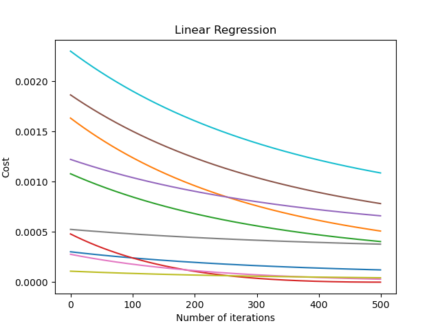
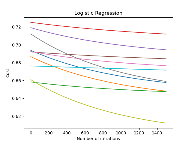
Original 2021 Training Curves
Note that each of the below two trainings was performed with 10 different values of initial theta. The initial value of theta effects the overall training performance. The best of the 10 was taken in consideration for the final evaluation on the test dataset.
Original 2021 Test Output
Linear Regression:
Test accuracy: 0.7068965517241379 .Test cost: 0.14745936729023856

Logistic Regression:
Test accuracy: 0.646551724137931 .Test cost: 0.2865915372479961
Assimilated code
Additional Notes
- The example does not use regularization or missing-value imputation.
- Select parameters using validation data, then evaluate the selected model on held-out test data.
- Squared loss and cross-entropy have different meanings; their raw values are not directly comparable.
- The archived plots do not establish that one algorithm is better. A new comparison needs the corrected pipeline and a consistent evaluation protocol.
Have a question or a different approach? I’d like to hear it.
Comments
Comments load as you reach this section. Sign in with GitHub to join.
Read or comment on GitHub ↗